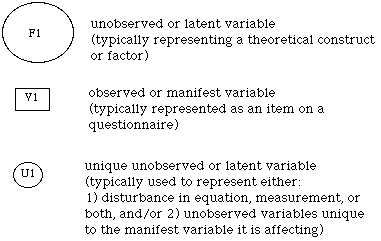
Figure 1. Standard conventions for representing variables.
Feel free to send comments to: wchin@uh.edu
originally created: November 28, 1995
last update: November 29, 1995
In Figure 2, a single factor model is presented. The latent variable
F1 is assumed to have a variance of one since no asterisk is assigned to
it. Three manifest variables (V1 through V3) are presented and assumed
to reflect the underlying factor. The extent to which these measured items
actually tap into the underlying factor are determined by estimating their
respective path loadings (P1* through P3*). Finally, the model indicates
that each manifest variable may also measure other factors beyond the particular
one of interest. Alternatively, there may be a certain amount of measurement
error reflected in each manifest variable. This assumption is modeled by
having each manifest variable affected by a unique factor (U1* through
U3*). In the figure, the path loadings from each unique factor are fixed
at 1 with the variance of each unique factor needing to be estimated (as
indicated by an asterisk). An alternative approach would be to fix the
variances for each unique factor to 1 and estimate the corresponding paths.
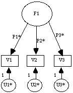
Figure 2: A single factor model.
Note that in the model presented, it is not enough to diagram the paths among factors and manifest variables. Such path diagrams are often presented in IS papers without indicating which parameters are being estimated and which are set at particular values. While the path diagrams among latent and manifest variables help convey the general ideas behind causal models, there is still enough information left out to make it difficult for other researchers to reproduce the analysis.
2.1.2.2. Population demographics
2.1.2.3. Statistical description (skewness, kurtosis - univariate and multivariate; outliers)
2.1.2.4. Number of subjects
2.1.2.5. Sample covariance matrix
2.2.2. For all correlated first order factors - two indicators per factor.
2.2.3. For orthogonal factors model - each factor must have three indicators (Anderson and Rubin, 1956)
2.2.4. If no rules are available - determine identification via algebraic manipulation.
2.2.5. Scale Indeterminacy (failure to set the metric associated with each factor)
2.3.2. Starting values used for estimation
2.3.3. Computational procedure employed (i.e., ML, ULS, GLS, WLS) consistent with the data?
2.3.4. Anomalies encountered during estimation
2.3.4.1. Were there improper solutions such as negative variances, standardized paths greater than +1 or -1?
2.3.4.2. Did the program set offending (i.e., negative) variances to zero?
2.3.5. Are the results presented confirmatory or exploratory?
2.4.2. Incremental fit indices: extent to which the specified model performs better than a baseline model (e.g., no underlying factors) (Bentler-Bonnet Normed Fit, Tucker-Lewis) .
2.4.3. Parsimonious fit: accounts for the degrees of freedom necessary to achieve the fit (Normed Chi-Square (Chi-Square/df), AGF, Akaike information criterion
2.4.4. Resampling Procedures
2.4.5.1.2. B) If the model is false, the chi-squared test statistic should be significant
2.4.5.1.3. Need appropriate power in order to ensure that statement B occurs.
2.4.5.2.2. the effect size of the path(s) for the correct model
2.4.5.2.3. number of indicators used
2.4.5.2.4. the alternative model used as a basis of comparison
2.4.5.3.3. 3) Take the resulting covariance matrix and analyze it using the original model (stipulating the sample size to be the same as the original model).
2.4.5.3.4. 4) The Likelihood ratio value (l) resulting from this analysis (i.e., the chi-square statistic from the program) should approximate a non-central chi-square distribution with degrees of freedom equal to the difference between the two models (Ho-Ha).